More than you want to know about air resistance, drag coefficient, velocity loss, and reaction time in baseball vs softball.

« By the time the ball crosses home plate, a pitch loses about 10 percent of its speed because of air resistance »

You probably heard the quote above a million times before. But how do we know this exactly? How do we know the velocity of a baseball as a function of time or distance traveled? Is it the same for softballs? What are the variables that play a role in the fractional loss of velocity? In this post, we are going to go over all this in great detail.*

(*yes, that means some math equations, but nothing a first-year STEM student shouldn’t be able to handle. But if you are not a math person, don’t worry, you can skip calculus stuff and go straight to the red equation in a box below and still get most of it.)

We all have a basic intuitive understanding of what drag is. We all understand that for the ball to go through the air, it must push it around to make its way, slowing down in the process. Many years ago, a wise man called Isaac Newton taught us that if an object changes its velocity, then there must be a force acting on it. More specifically, Newton’s second law of motion states that the force is always equal to the change in momentum per unit of time, i.e.

$\begin{equation*} \textbf{F} = \frac{\Delta \textbf{p}}{\Delta t} \end{equation*}$

where $\textbf{p}$ is the momentum (= $m\textbf{v}$ , the product of the mass and the velocity).

The force responsible for slowing down an object moving in a medium (air, water, etc.) is called the drag force. So what is the drag force due to air molecules interacting with a moving ball? Instead of looking at this as a ball moving through a stationary fluid (air), it is often easier to think about drag force in a reference frame where the ball is stationary and the fluid is moving at the speed v of the ball (this is completely equivalent). Imagine now that each time an air molecule hits the ball, its velocity goes to zero. Here is a simple animation showing what it looks like.

Click on the triangle to start animation (may not work well on a smartphone)

Since momentum is a conserved quantity, the molecule’s momentum must be transferred to the ball. The total change in momentum for the ball is thus simply the sum of the momentum of all the molecules that collided with the ball (the ones in red in the animation). It is easy to see that during a time interval $\Delta t$ , the total mass that has hit the ball will be equal to the volume of the cylinder swept by the ball (i.e. length $v\Delta t$ times cross-sectional area $A = \pi R^2$ where R is the ball’s radius) times the density of the air, $\rho$ . The change in the ball’s momentum is thus, by definition, mass times $v$ , i.e. $A \rho v^2\Delta t$ . Then, from the definition of the force given above, we obtain the following expression for the magnitude of the drag force:

$\begin{equation*} F_D = \frac{A \rho v^2\Delta t}{\Delta t} = A \rho v^2 \end{equation*}$

We thus see that the drag force is proportional to the density of air, the square of the radius, and the square of the velocity. Of course, in reality, things are a bit more complicated than this simple model. Air molecules do not all completely stop after a collision (they are pushed around) and only a fraction of each molecule’s momentum is transferred to the ball. To account for this, we say that on average, a fraction $\frac{1}{2} C_D$ of the momentum is transferred to the ball, where $C_D$ is the so-called drag coefficient. The drag force is thus usually expressed with this simple formula:

$\begin{equation*} F_D = \frac{1}{2} C_D A \rho v^2 \end{equation*}$

The value of $C_D$ is not a constant but varies as a function of the flow speed, flow direction, object position, object size, fluid density, and fluid viscosity. For some simple geometries, it can be calculated from first principles, but it is usually determined empirically from wind tunnel experiments or other direct measurements or estimated from numerical simulations. To give an idea, for a smooth sphere, $C_D$ is around 0.5 depending on the velocity. If you add elements of roughness, such as seams or a scuff on a baseball, $C_D$ becomes much lower but determining its exact value is complicated (believe me, I have been playing in this rabbit hole for a while now). Anyhow, if somehow you know the drag coefficient, then you know the drag force and you are in business to calculate stuff.

One of the first things every student of physics learns after being introduced to Newton’s laws is to calculate the motion of a projectile when air resistance is negligible. This is an easy problem that can be solved in only a few lines of calculation on a piece of paper. Unfortunately, if you add a force that is proportional to $v^2$ , the equations of motion can no longer be solved analytically and numerical techniques are required to obtain the full trajectory.

However, in the particular case when the only force acting on an object is the drag force (i.e. we neglect gravity and other aerodynamic forces), it is still possible to solve the equations exactly. In that situation, since the only acting force is parallel to the velocity, the object will move in a straight line with a deceleration that will depend on the magnitude of the instantaneous drag force. To find the velocity of the ball during its flight, we need to solve a differential equation that is obtained by simply applying Newton’s second law, that is setting the mass times the acceleration of the ball equal to the drag force:

$\begin{equation*} m\frac{dv}{dt} = -\frac{1}{2} C_D A \rho v^2 \end{equation*}$

where the minus sign indicates that the force acts in a direction opposite to the velocity, thus slowing it down. The equation can easily be rearranged to obtain

$\begin{equation*} \frac{dv}{v^2} = -\frac{C_D\rho A}{2m} dt \end{equation*}$

Integrating with the limits that the initial velocity is $v_0$ and at a later time $t$ the velocity is $v$

$\begin{equation*} \int_{v_0}^v \frac{dv'}{v'^2} = -\frac{C_D\rho A}{2m} \int_0^t dt' \end{equation*}$

we finally get that the velocity as a function of time is given by

$\begin{equation*} v(t) = \frac{1}{ \frac{1}{v_0} + \frac{C_D\rho At}{2m} } = \frac{v_0}{ 1+ \frac{v_0C_D\rho At}{2m} } \end{equation*}$

While this equation gives you exactly the velocity as a function of time, it does not tell you what will the velocity be after traveling a distance $D$ . For that, we need to know the time it takes to travel that distance and plug it into the equation. During a time $dt$ , an object with velocity $v(t)$ will travel a distance $ds = v(t)dt$ . Integrating on both sides

$\begin{equation*} \int_0^D ds = \int_0^t v(t')dt' \end{equation*}$

we obtain a relationship between the travelled distance $D$ and the time of flight $t$ :

$\begin{equation*} D = \int_0^t \frac{v_0}{ 1+ \frac{v_0C_D\rho At'}{2m} } dt' = \ln \Big(1 +\frac{v_0C_D\rho At}{2m} \Big) /\Big(\frac{C_D\rho A}{2m}\Big) \end{equation*}$

The time to travel this distance $D$ is then easily obtained from isolating $t$ in the above equation:

$\begin{equation*} t(D) =\frac{ \exp\Big(\frac{DC_D\rho A}{2m}\Big) - 1 }{\frac{v_0C_D\rho A}{2m} }\end{equation*}$

Plugging this time of travel into the equation for $v(t)$ , everything simplifies quite nicely to provide this simple expression for the final velocity

The exponential term tells you exactly how much of the initial velocity has been lost due to drag. Let’s put some numbers into it. Air density is typically 1.2 kg/m $^3$ although it changes with variation in atmospheric pressure, altitude, temperature, and density. For a typical baseball with a circumference of 9.125 inches (or 3.688 cm radius), a mass of 5.125 ounces (145.29 g), assuming a drag coefficient of 0.35 (see historical values here) and a distance of $D$ = 55 ft (16.764 m) the exponential term is equal to 0.9016. In other words, after a travel of 55 ft, the velocity of the ball is 90% of its initial value (give or take a bit depending on the exact value of the local air density and size and mass of your ball). So the quote at the top of this post is correct…unless you are in Denver, in which case the ball only loses about 8.5% of its velocity because of the thinner air (about 1.02 kg/m $^3$ ). So a 95 mph fastball’s final velocity in Denver will end 1.35 mph faster than at sea level (this is as if, in terms of reaction time, the ball was thrown at 95.8 mph at sea level).

What about a softball? A softball is larger and heavier than a baseball. It is also thrown at about two-thirds of typical MLB fastballs. However, softball pitchers release the ball about 37 ft from the home plate so it has less time to slow down. Given that, what fraction of its initial velocity is lost due to air drag? For a typical softball with a circumference of 12 inches (or 4.851 cm radius), a mass of 6.625 ounces (187.82 g), and assuming the same drag coefficient as for a baseball (check this), for a distance $D = 37$ ft (16.764 m) the exponential term is 0.91099, only a 1% difference with the value found for a baseball. In other words, the difference in mass and radius almost compensate completely for the difference in traveled distance in terms of fractional velocity loss.

If you are interested to know the difference in reaction time between a fastball from Jacob deGrom vs Jennie Finch, below is a simple calculator that does that for you (feel free to change the assumed values for the mass/radius/distance/air density if you don’t like them).

Click on the triangle to start the program. Click on the pencil icon to change the values to your preferred ones.

Similarly, here is a plot showing the baseball velocity needed to have the same reaction time as a softball pitch.

Click on the triangle to start the program.

Note that this is an exact result, no approximations have been made in the derivation of these equations. However, this is valid only for the case where the only force acting on the ball is in the same (or in this case, the opposite) direction as the velocity. For real baseballs, other forces are acting in other directions (gravity, Magnus, and non-Magnus) which will deviate the trajectory from a straight line.

But given that the deviation from a straight line is at most a few feet (up/down or left/right) compared to a total travel length of about 55 ft, maybe this little 1D model is not bad after all. Let’s check that out in detail.

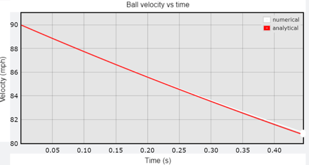
Ironically, calculating the whole 3D trajectory numerically is actually easier than what I just presented above (it’s so simple that even a computer can do it!). Using my trajectory simulator, but modified for pitched balls, I can calculate the velocity as a function of time for various type of pitches and compare it to what our little analytic formula predicts. The figure below shows that for a 90 mph fastball with a spin of 2500 rmp, the final velocities with the two approach differ by only 0.1%. And at 100 mph, the agreement reaches 0.06%. Not bad at all! The small difference is of course due to the fact that the numerical simulation includes the Magnus force and gravity (although they partially cancel out, gravity wins and the ball falls by about a foot. There is no such thing as a rising fastball!). For a curveball, the difference grows to close to 1% since the ball falls quite a lot more. Of course, if I turn off the gravity and Magnus forces, then there is an almost perfect match (0.001%, the tiny difference being due to the finite time step of 0.001s used in the numerical calculations).

Fig 1. Numerical vs analytical velocity of a baseball as a function of time for a 90 mph/2500 rpm fastball.

Now that we know that the simple analytical expression works pretty well for fastballs, one could, in principle, measure the drag coefficient provided you know the velocity of the ball at two points separated by a distance $D$ . Indeed, from the equation in the box above, we obtain

$\begin{equation*} C_D = \Big(\frac{-2m}{D\rho A} \Big)\ln(v_f/v_0) \end{equation*}$

were $v_0$ and $v_f$ are the initial and final velocities.

Hence, in theory, the drag coefficient could easily be measured provided one has access to the full details of a trajectory. Unfortunately, I do not have privileged access to Hawkeye data to test this. Would such an approach be much better than the one used here (based on the method described here)? I suspect that the details of the method used do not matter that much as the error on such measurements is probably dominated by the radii/mass variations from ball to ball (not to mention the exact determination of the local air density). Perhaps a more precise way of doing things would be to ask a pitcher to throw dozen of pitches using the same ball that has been carefully measured beforehand instead of using game data. Anyhow, I think we are very lucky to live in an era when technological advances allow us to tackle in great detail all the intricacies of baseball trajectories.

If you made it this far, let me know, you definitely earned bragging rights in the comment section.

Laisser un commentaire Annuler la réponse